Solved Problem on RLC Circuits
advertisement
A series RLC circuit contains a resistor with resistance R = 75 Ω, an inductor with
inductance L = 10 mH, and a capacitor with capacitance C = 0.20 μF. The initial charge stored
in the capacitor is equal to q0 = 0.4 mC and the current is zero. Determine:
a) The equation of electric charge as a function of time;
b) What is the type of oscillations in this circuit;
c) The graph of charge q versus time t.
a) The equation of electric charge as a function of time;
b) What is the type of oscillations in this circuit;
c) The graph of charge q versus time t.

Problem data:
- Capacitance: C = 0.20 μF;
- Resistance: R = 75 W;
- Inductance: L = 10 mH;
- Initial charge stored in the capacitor: q0 = 0.4 mC;
- Initial current: I0 = 0.
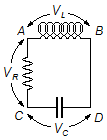
From the initial instant, a current begins to circulate, and the charge on the capacitor decreases while
the current in the circuit increases, in each element of the circuit we have a potential difference
(Figure 1). With this, we write the Initial Conditions of the problem
\[
\begin{gather}
q(0)=q_{0}\\[10pt]
i_{0}=\frac{dq(0)}{dt}=0
\end{gather}
\]
Solution
a) Applying Kirchhoff's Second Law (Figure 1)
\[
\begin{gather}
\bbox[#99CCFF,10px]
{\sum_{i=1}^{n}V_{i}=0} \tag{I}
\end{gather}
\]
Between points A and B, we have a potential difference in the inductor given by
\[
\begin{gather}
\bbox[#99CCFF,10px]
{V_{L}=L\frac{di}{dt}} \tag{II}
\end{gather}
\]
between points C and D, we have a potential difference in the capacitor given by
\[
\begin{gather}
\bbox[#99CCFF,10px]
{V_{C}=\frac{q}{C}} \tag{III}
\end{gather}
\]
between points A and C, we have a potential difference in the resistor given by
\[
\begin{gather}
\bbox[#99CCFF,10px]
{V_{R}=Ri} \tag{IV}
\end{gather}
\]
substituting expressions (II), (III), and (IV) into expression (I)
\[
\begin{gather}
V_{L}+V_{R}+V_{C}=0\\[5pt]
L\frac{di}{dt}+Ri+\frac{q}{C}=0
\end{gather}
\]
the instantaneous current is given by
\[
\begin{gather}
\bbox[#99CCFF,10px]
{i=\frac{dq}{dt}}
\end{gather}
\]
\[
\begin{gather}
L\frac{d}{dt}\left(\frac{dq}{dt}\right)+R\frac{dq}{dt}+\frac{q}{C}=0\\[5pt]
L\frac{d^{2}q}{dt^{2}}+R\frac{dq}{dt}+\frac{q}{C}=0
\end{gather}
\]
this is a Second-Order Homogeneous Ordinary Differential Equation. Dividing the equation by the
inductance L
\[
\begin{gather}
\frac{d^{2}q}{dt^{2}}+\frac{R}{L}\frac{dq}{dt}+\frac{1}{LC}q=0
\end{gather}
\]
substituting the values given in the problem
\[
\begin{gather}
\frac{d^{2}q}{dt^{2}}+\frac{75}{10\times10^{-3}}\frac{dq}{dt}+\frac{1}{10\times10^{-3}\times0.20\times10^{-6}}q=0\\[5pt]
\frac{d^{2}q}{dt^{2}}+\frac{75}{10^{-2}}\frac{dq}{dt}+\frac{1}{2\times10^{-9}}q=0\\[5pt]
\frac{d^{2}q}{dt^{2}}+7.5\times10^{3}\frac{dq}{dt}+5\times10^{8}q=0 \tag{V}
\end{gather}
\]
Solution of \( \displaystyle \frac{d^{2}q}{dt^{2}}+7.5\times10^{3}\frac{dq}{dt}+5\times10^{8}q=0 \)
The solution to this type of equation is found substituting
Differentiation of the expression (VI) with respect to time
The solution to this type of equation is found substituting
\[
\begin{gather}
q=\operatorname{e}^{\lambda t}\\[5pt]
\frac{dq}{dt}=\lambda \operatorname{e}^{\;\lambda t}\\[5pt]
\frac{d^{2}q}{dt^{2}}=\lambda ^{2}\operatorname{e}^{\lambda t}
\end{gather}
\]
substituting these values into the differential equation
\[
\begin{gather}
\lambda^{2}\operatorname{e}^{\lambda t}+7.5\times10^{3}\lambda \operatorname{e}^{\lambda t}+5\times10^{8}\operatorname{e}^{\lambda t}=0\\[5pt]
\operatorname{e}^{\lambda t}\left(\lambda ^{2}+7.5\times10^{3}\lambda +5\times10^{8}\right)=0\\[5pt]
\lambda^{2}+7.5\times10^{3}\lambda +5\times10^{8}=\frac{0}{\operatorname{e}^{\lambda t}}\\[5pt]
\lambda ^{2}+7.5\times10^{3}\lambda +5\times10^{8}=0
\end{gather}
\]
this is the Characteristic Equation that has a solution
\[
\begin{gather}
\Delta=b^{2}-4ac=\left(7.5\times10^{3}\right)^{2}-4.5\times10^{8}=5.63\times10^{7}-2.00\times10^{9}=-1.94\times10^{9}
\end{gather}
\]
for Δ<0 the roots are complex of the form a+bi, where
\( \mathsf{i}=\sqrt{-1\;} \)
\[
\begin{gather}
\lambda =\frac{-b+\sqrt{\Delta\;}}{2a}=\frac{-7.5\times10^{3}+\sqrt{-1.94\times10^{9}\;}}{2\times1}=-{\frac{-7.5\times10^{3}\pm4.4\times10^{4}\mathsf{i}}{2}}\\[5pt]
\lambda_{1}=-3.75\times10^{3}+2.20\times10^{4}\mathsf{i}\qquad \text{e}\qquad \lambda_{2}=-3.75\times10^{3}-2.20\times10^{4}\mathsf{i}
\end{gather}
\]
The solution to the differential equation will be
\[
\begin{gather}
q=C_{1}\operatorname{e}^{\lambda_{1}t}+C_{2}\operatorname{e}^{\lambda_{2}t}\\[5pt]
q=C_{1}\operatorname{e}^{\left(-3.75\times10^{3}+2.20\times10^{4}\mathsf{i}\right)t}+C_{2}\operatorname{e}^{\left(-3.75\times10^{3}-2.20\times10^{4}\mathsf{i}\right)t}\\[5pt]
q=C_{1}\operatorname{e}^{\left(-3.75\times10^{3}t+2.20\times10^{4}\mathsf{i}t\right)}+C_{2}\operatorname{e}^{\left(-3.75\times10^{3}t+2.20\times10^{4}\mathsf{i}t\right)}\\[5pt]
q=C_{1}\operatorname{e}^{-3.75\times10^{3}t}\operatorname{e}^{2.15\times10^{4}\mathsf{i}t}+C_{2}\operatorname{e}^{-3.75\times10^{3}t}\operatorname{e}^{-2.15\times10^{4}\mathsf{i}t}\\[5pt]
q=\operatorname{e}^{-3.75\times10^{3}t}\left(C_{1}\operatorname{e}^{2.20\times10^{4}\mathsf{i}t}+C_{2}\operatorname{e}^{-2.20\times10^{4}\mathsf{i}t}\right)
\end{gather}
\]
where C1 and C2 are constants of integration, using
Euler's Formula
\( \operatorname{e}^{\mathsf{i}\theta }=\cos \theta +\mathsf{i}\sin \theta \)
\[
\begin{gather}
q=\operatorname{e}^{-3.75\times10^{3}t}\left[C_{1}\left(\cos2.20\times10^{4}t+\mathsf{i}\sin 2.20\times10^{4}t\right)+C_{2}\left(\cos2.20\times10^{4}t-\mathsf{i}\sin 2.20\times10^{4}t\right)\right]\\[5pt]
q=\operatorname{e}^{-3.75\times10^{3}t}\left(C_{1}\cos2.20\times10^{4}t+\mathsf{i}C_{1}\sin 2.20\times10^{4}t+C_{2}\cos2.20\times10^{4}t-\mathsf{i}C_{2}\sin 2.20\times10^{4}t\right)\\[5pt]
q=\operatorname{e}^{-3.75\times10^{3}t}\left[\left(C_{1}+C_{2}\right)\cos2.20\times10^{4}t+\mathsf{i}\left(C_{1}-C_{2}\right)\sin 2.20\times10^{4}t\right]
\end{gather}
\]
defining two new constants α and β in terms of C1 and
C2
\[
\begin{gather}
\alpha \equiv C_{1}+C_{2}\\[5pt]
\text{e}\\[5pt]
\beta \equiv \mathsf{i}(C_{1}-C_{2})
\end{gather}
\]
\[
\begin{gather}
q=\operatorname{e}^{-3.75\times10^{3}t}\left(\alpha \cos 2.20\times10^{4}t+\beta\sin 2.20\times10^{4}t\right) \tag{VI}
\end{gather}
\]
where α and β are constants determined by the Initial Conditions.
Differentiation of the expression (VI) with respect to time
\[
\begin{gather}
q=\underbrace{\operatorname{e}^{-3.75\times 10^{3}t}}_{u}\underbrace{\left(\alpha\cos 2.20\times 10^{4}t+\beta \sin 2.20\times 10^{4}t\right)}_{v}
\end{gather}
\]
using the Product Rule for the differentiation of functions
\[
\begin{gather}
(uv)'=u'v+uv'
\end{gather}
\]
where
\( u=\operatorname{e}^{-3.75\times 10^{3}t} \)
and
\( v=\left(\alpha \cos 2.20\times 10^{4}t+\beta\sin 2.20\times 10^{4}t\right) \),
the term in parentheses is a sum of functions, the derivative is given by the sum of the derivatives
\[
\begin{gather}
(f+g)'=f'+g'
\end{gather}
\]
and the functions sine and cosine are composite functions, using the Chain Rule
\[
\begin{gather}
\frac{df[w(t)]}{dt}=\frac{df}{dw}\frac{dw}{dt}
\end{gather}
\]
with
\( f=\alpha \cos w \),
\( g=\beta \sin w \)
and
\( w=2.20\times 10^{4}t \)
\[
\begin{gather}
\frac{dx}{dt}=\frac{du}{dt}v+u\frac{dv}{dt}\\[5pt]
\frac{dx}{dt}=\frac{du}{dt}v+u\left(\frac{df}{dt}+\frac{dg}{dt}\right)\\[5pt]
\frac{dx}{dt}=\frac{du}{dt}v+u\left(\frac{df}{dw}\frac{dw}{dt}+\frac{dg}{dw}\frac{dw}{dt}\right)\\[5pt]
\frac{dx}{dt}=\frac{d(\operatorname{e}^{-3.75\times 10^{3}t})}{dt}\left(\alpha\cos 2.20\times 10^{4}t+\beta\sin 2.20\times 10^{4}t\right)+\\
+(\operatorname{e}^{-3.75\times 10^{3}t})\left[\frac{d(\alpha\cos w)}{dw}\frac{d(2.20\times 10^{4}t)}{dt}+\frac{d(\beta\sin w)}{dw}\frac{d(2.20\times 10^{4}t)}{dt}\right]\\[5pt]
\frac{dx}{dt}=-3.75\times 10^{3}\operatorname{e}^{-3.75\times 10^{3}t}\left(\alpha\cos 2.20\times 10^{4}t+\beta\sin 2.20\times 10^{4}t\right)+\\
+(\operatorname{e}^{-3.75\times 10^{3}t})\left[(-\alpha\sin (2.20\times 10^{4})(2.20\times 10^{4})+(\beta \cos w)(2.20\times 10^{4})\right]\\[5pt]
\frac{dx}{dt}=\operatorname{e}^{-3.75\times 10^{3}t}\left[\left(-3.75\times 10^{3}\alpha\cos 2.20\times 10^{4}t-3.75\times 10^{3}\beta\sin 2.20\times 10^{4}t\right)\right.+\\
+\left.\left(-2.20\times 10^{4}\alpha\sin 2.20\times 10^{4}t+2.20\times 10^{4}\beta \cos2.20\times 10^{4}t\right)\right]\\[5pt]
\frac{dx}{dt}=\operatorname{e}^{-3.75\times 10^{3}t}\left[\left(-3.75\times 10^{3}\alpha\cos 2.20\times 10^{4}t-2.20\times 10^{4}\alpha\sin 2.20\times 10^{4}t\right)\right.+\\
+\left.\left(-3.75\times 10^{3}\beta\sin 2.20\times 10^{4}t+2.20\times 10^{4}\beta \cos2.20\times 10^{4}t\right)\right]\\[5pt]
\frac{dx}{dt}=\operatorname{e}^{-3.75\times 10^{3}t}\left[-\alpha\left(3.75\times 10^{3}\cos2.20\times 10^{4}t+2.20\times 10^{4}\sin 2.20\times 10^{4}t\right)\right.+\\
+\left.\beta\left(2.20\times 10^{4}\cos2.20\times 10^{4}t-3.75\times 10^{3}\sin 2.20\times 10^{4}t\right)\right] \tag{VII}
\end{gather}
\]
Substituting the Initial Conditions into expressions (VI) and (VII)
\[
\begin{gather}
x(0)=4\times 10^{-4}=\operatorname{e}^{-3.75\times 10^{3}\times 0}\left(\alpha\cos 2.20\times 10^{4}\times 0+\beta \sin 2.20\times 10^{4}\times 0\right)\\[5pt]
\alpha=4\times 10^{-4} \tag{VIII}
\end{gather}
\]
\[
\begin{gather}
\frac{dx(0)}{dt}=0=\operatorname{e}^{-3.75\times 10^{3}\times 0}\left[-4\times 10^{-4}\times\left(3.75\times 10^{3}\cos2.20\times 10^{4}\times 0+2.20\times 10^{4}\sin 2.20\times 10^{4}\times 0\right)\right.+\\
+\left.\beta\left(2.20\times 10^{4}\cos2.20\times 0-3.75\times 10^{3}\sin 2.20\times 10^{4}\times 0\right)\right]\\[5pt]
0=-4\times 10^{-4}\times\left(3.75\times 10^{3}\times 1+0\right)+\beta\left(2.20\times 10^{4}\times 1-0\right)\\[5pt]
1.50=2.20\times 10^{4}\beta \\[5pt]
\beta=\frac{1.50}{2.20\times 10^{4}}\\[5pt]
\beta =6\times 10^{-5} \tag{IX}
\end{gather}
\]
substituindo as constantes (VIII) e (IX) na expressão (VI)
\[
\begin{gather}
q=\operatorname{e}^{-3.75\times 10^{3}t}\left(4\times 10^{-4}\cos2.20\times 10^{4}t+6\times 10^{-5}\sin 2.20\times 10^{4}t\right)
\end{gather}
\]
Equation of charge
\[
\begin{gather}
\bbox[#FFCCCC,10px]
{q(t)=\operatorname{e}^{-3.75\times 10^{3}t}\left(4\times 10^{-4}\cos2.20\times 10^{4}t+6\times 10^{-5}\sin 2.20\times 10^{4}t\right)}
\end{gather}
\]
b) As Δ<0 this is an underdamped RLC circuit oscillator.
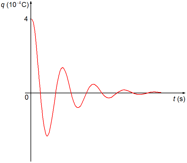
c) Plotting the graph of
\[
\begin{gather}
q(t)=\operatorname{e}^{-3.75\times 10^{3}t}\left(4\times 10^{-4}\cos2.20\times 10^{4}t+6\times 10^{-5}\sin 2.20\times 10^{4}t\right)
\end{gather}
\]
The function q(t) is the product of two functions,
\( f(t)=\operatorname{e}^{-3.75\times 10^{3}t} \)
and
\( g(t)=4\times 10^{-4}\cos 2.20\times 10^{4}t+6\times 10^{-5}\sin 2.20\times 10^{4}t \).
To find the roots we set q(t) = 0, as
q(t) = f(t)g(t) we have f(t) = 0 or
g(t) = 0.
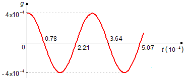
- For g(t) = 0
\[
\begin{gather}
g(t)=4\times 10^{-4}\cos2.20\times 10^{4}t+6\times 10^{-5}\sin 2.20\times 10^{4}t=0\\[5pt]
6\times 10^{-5}\sin 2.20\times 10^{4}t=-4\times 10^{-4}\cos2.20\times 10^{4}t\\[5pt]
\frac{\sin 2.20\times 10^{4}t}{\cos2.20\times 10^{4}t}=-{\frac{4\times 10^{-4}}{6\times 10^{-5}}}\\[5pt]
\tan 2.20\times 10^{4}t=-6.67\\[5pt]
2.20\times 10^{4}t=\arctan(-6.67)\\[5pt]
t=\frac{1}{2.20\times 10^{4}}\left[-\arctan(6.67)+n\pi\right]\\[5pt]
t=\frac{1}{2.20\times 10^{4}}\left[-1.42+n\pi \right]
\end{gather}
\]
for these values of t, we have the roots of the function g(t), the first four values
for n = 0, 1, 2, and 3 will be t = 0.78×10⁻⁴; 2.21×10⁻⁴;
3.64×10⁻⁴ and 5.07×10⁻⁴ (Graph 1).
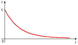
- For f(t) = 0
\[
\begin{gather}
f(t)=\operatorname{e}^{-3.75\times 10^{3}t}=0\\[5pt]
\operatorname{e}^{-3.75\times 10^{3}t}=0
\end{gather}
\]
as there is no t that satisfies this equality, the function f(t) does not intersect
the t-axis. For any real value of t the function will always be positive,
f(t) > 0.Differentiation of the expression f(t)
\[
\begin{gather}
\frac{df}{dt}=-3.75\times 10^{3}\operatorname{e}^{-3.75\times 10^{3}t}
\end{gather}
\]
for any real value of t, the derivative will always be negative
\( \left(\frac{df(t)}{dt}<0\right) \)
and the function always decreases. Setting
\( \frac{df(t)}{dt}=0 \)
we find the maximum and minimum points of the function.
\[
\begin{gather}
\frac{df}{dt}=-3.75\times 10^{3}\operatorname{e}^{-3.75\times 10^{3}t}=0\\[5pt]
\operatorname{e}^{-3.75\times 10^{3}t}=\frac{0}{-3.75\times 10^{3}}\\[5pt]
\operatorname{e}^{-3.75\times 10^{3}t}=0
\end{gather}
\]
as there is no t that satisfies this equality, there are no maximum or minimum points of the
function.The second derivative of the expression f(t)
\[
\begin{gather}
\frac{d^{2}f}{dt^{2}}=-3.75\times 10^{3}(-3.75\times 10^{3})\operatorname{e}^{-3.75\times 10^{3}t}\\[5pt]
\frac{d^{2}f}{dt^{2}}=1.41\times 10^{7}\operatorname{e}^{-3.75\times 10^{3}t}
\end{gather}
\]
for any value of real t, the second derivative will always be positive
\( \left(\frac{d^{2}f(t)}{dt^{2}}>0\right) \)
and the function is concave upward. Setting
\( \frac{d^{2}f(t)}{dt^{2}}=0 \)
we find inflection points in the function.
\[
\begin{gather}
\frac{d^{2}f}{dt^{2}}=1.41\times 10^{7}\operatorname{e}^{-3.75\times 10^{3}t}=0\\[5pt]
\operatorname{e}^{-3.75\times 10^{3}t}=\frac{0}{1.41\times 10^{7}}\\[5pt]
\operatorname{e}^{-3.75\times 10^{3}t}=0
\end{gather}
\]
as there is no t that satisfies this equality, there are no inflection points in the function.For t = 0 the value f(0) will be
\[
\begin{gather}
f(0)=\operatorname{e}^{-3.75\times 10^{3}\times 0}\\[5pt]
f(0)=\operatorname{e}^{-0}\\[5pt]
f(0)=1
\end{gather}
\]
As the variable t represents time, we do not calculate negative values, t < 0, for
t tending to infinity
\[
\begin{gather}
\lim_{t\rightarrow \infty }f(t)=\lim _{t \rightarrow \infty}\operatorname{e}^{-3.75\times 10^{3}t}=\lim_{t\rightarrow \infty}{\frac{1}{\operatorname{e}^{3.75\times 10^{3}t}}}=\lim_{t\rightarrow \infty}{\frac{1}{\operatorname{e}^{\infty }}}=0
\end{gather}
\]
From the above analysis, we plotted the graph of f versus t (Graph 2).
As q(t) = f(t)g(t), the combination of graphs produces a curve that oscillates like the cosine function damped by the exponential (Graph 3).
advertisement

Fisicaexe - Physics Solved Problems by Elcio Brandani Mondadori is licensed under a Creative Commons Attribution-NonCommercial-ShareAlike 4.0 International License .