Solved Problem on Static Equilibrium

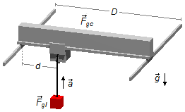
A crane with weight F_gc, the distance between the rails in which it is supported is D. A load with weight F_gl lies at a distance d from one of the rails. Determine the reaction force of the crane on the rails by lifting the load with an acceleration a=g, where g is the acceleration due to gravity.

Problem data:

Crane weight: W=F_gc;
Load weight: F_gl;
Distance between crane rails: D;
Distance from load to one of the rails: d;
Acceleration of load rising: g;
Acceleration due to gravity: g.

Problem diagram:

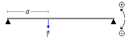
In the load acts, the gravitational force \( {\vec F}_{gc} \), and the tension force \( \vec{T} \), the tension is transmitted by the rope to the crane (Figure 1-A).

Figure 1

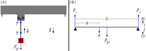
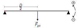
This system is equivalent to a bar supported at the ends, of gravitational force \( {\vec F}_{gc} \) equal to the weight of the crane at the center in point \( \frac{D}{2} \). The tension force \( \vec{T} \) in the cord due to the load acts at a distance d from one end. The reaction forces \( {\vec F}_{1} \) and \( {\vec F}_{2} \) are applied at the end of the bar. We assume the counterclockwise direction as positive (Figure 1-B).
We choose a reference frame at the point where is the reaction force \( {\vec F}_{1} \).

Solution

Drawing a free-body diagram we have the forces that act on it, we can apply Newton's Second Law

\[ \begin{gather} \bbox[#99CCFF,10px] {\vec{F}=m\vec{a}} \end{gather} \]

Assuming the positive direction upwards (Figure 2)

\[ \begin{gather} T-F_{gl}=ma \tag{I} \end{gather} \]

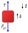
Figure 2

where m is the mass of the load, the gravitational force due to the load is given by

\[ \begin{gather} F_{gl}=ma \end{gather} \]

the mass will be

\[ \begin{gather} m=\frac{F_{gl}}{a} \tag{II} \end{gather} \]

substituting the expression (II) into expression (I)

\[ \begin{gather} T-F_{gl}=\frac{F_{gl}}{\cancel{a}}\,\cancel{a}\\[5pt] T-F_{gl}=F_{gl}\\[5pt] T=F_{gl}+F_{gl}\\[5pt] T=2F_{gl} \tag{III} \end{gather} \]

For the bar remains in equilibrium we must have the following conditions

\[ \begin{gather} \bbox[#99CCFF,10px] {\sum F_{i}=0} \tag{IV-a} \end{gather} \]

\[ \begin{gather} \bbox[#99CCFF,10px] {\sum {\Large\tau}_{i}=0} \tag{IV-b} \end{gather} \]

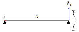
Drawing the forces that act on the bar in a coordinate system xy (Figure 3) and applying the condition of (IV-a)

\[ \begin{gather} F_{1}+F_{2}-T-F_{gc}=0 \end{gather} \]

substituting the expression (III)

\[ \begin{gather} F_{1}+F_{2}-2F_{gl}-F_{gc}=0\tag{V} \end{gather} \]

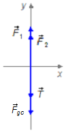
Figure 3

The torque of a force is given by

\[ \begin{gather} \bbox[#99CCFF,10px] {{\Large\tau}=Fd} \tag{VI} \end{gather} \]

Torque of reaction force \( {\vec{F}}_{1} \):

Applying the expression (V), we have the force F represented by the reaction force \( {\vec F}_{1} \) and the distance is equal to zero, d = 0, the reaction force is applied at the same point taken as a reference

\[ \begin{gather} {\Large\tau}_{{F}_{1}}=0 \tag{VII} \end{gather} \]

Torque of the tension force:

Applying the expression (V), we have the force F represented traction force \( \vec{T} \) which is applied at a point at a distance from the reference point, as it tends to make the bar rotate in the opposite direction of the reference the torque will be negative (Figure 4)

Figure 4

\[ \begin{gather} {\Large\tau}_{T}=-Td \tag{VII} \end{gather} \]

substituting the expression (III) into expression (VIII)

\[ \begin{gather} {\Large\tau}_{T}=-2F_{gl}d \tag{IX} \end{gather} \]

Torque of the gravitational force of the bar:

Applying the expression (V), we have the force F represented by the gravitational force of the bar \( {\vec F}_{gc} \) which is applied at the midpoint of the bar, as it tends to make the bar rotate against the direction of the reference the torque will be negative (Figure 5)

Figure 5

\[ \begin{gather} {\Large\tau}_{F_{gc}}=-F_{gc}\,\frac{D}{2} \tag{X} \end{gather} \]

Torque of reaction force \( {\vec{F}}_{2} \):

Applying the expression (V), we have the force F represented by the reaction force \( {\vec F}_{2} \) and the distance will be the length of the bar, d=D, as it tends to make the bar rotate in the same direction of the reference the torque will be positive (Figure 6)

Figure 6

\[ \begin{gather} {\Large\tau}_{{F}_{2}}=F_{2}D \tag{XI} \end{gather} \]

Applying the second condition (IV)

\[ \begin{gather} {\Large\tau}_{F_{1}}+{\Large\tau}_{T}+{\Large\tau}_{F_{gc}}+{\Large\tau}_{F_{2}}=0 \end{gather} \]

substituting the expression (VII) into the expressions (IX), (XI), and (XI)

\[ \begin{gather} 0-2F_{gl}d-F_{gc}\,\frac{D}{2}+F_{2}\,D=0\\[5pt] -2F_{gl}d-F_{gc}\,\frac{D}{2}+F_{2}\,D=0 \tag{XII} \end{gather} \]

Expressions (V) and (XII) can be written as a system of two equations to two variables F₁ and F₂

\[ \begin{gather} \left\{ \begin{array}{l} F_{1}+F_{2}-2F_{gl}-F_{gc}=0\\ -2F_{gl}d-F_{gc}\,\dfrac{D}{2}+F_{2}\,D=0 \end{array} \right.\ \end{gather} \]

from the second equation, we have the value of F₂

\[ \begin{gather} -2F_{gl}d-F_{gc}\,\frac{D}{2}+F_{2}\,D=0\\[5pt] F_{2}\,D=2F_{gl}d+F_{gc}\,\frac{D}{2} \end{gather} \]

\[ \begin{gather} \bbox[#FFCCCC,10px] {F_{2}=2F_{gl}\frac{d}{D}+\frac{F_{gc}}{2}} \end{gather} \]

substituting this value in the first equation

\[ \begin{gather} F_{1}+\frac{1}{D}\,\left(\,2F_{gl}d+F_{gc}\,\frac{D}{2}\,\right)-2F_{gl}-F_{gc}=0\\[5pt] F_{1}=-\frac{{1}}{D}\,\left(\,2F_{gl}d+F_{gc}\,\frac{D}{2}\,\right)+2F_{gl}+F_{gc}\\[5pt] F_{1}=-\frac{{1}}{D}\,2F_{gl}d-\frac{1}{D}\,F_{gc}\,\frac{D}{2}+2F_{gl}+F_{gc}\\[5pt] F_{1}=-2\,\frac{F_{gl}d}{D}+2F_{gl}-\frac{F_{gc}}{2}+F_{gc} \end{gather} \]

factoring 2F_gl on the first and second terms on the right-hand side of the equation, and multiplying and dividing the fourth term by 2

\[ \begin{gather} F_{1}=2\,F_{gl}\,\left(\,-\frac{d}{D}+1\,\right)-\frac{F_{gc}}{2}+F_{gc}\times\frac{2}{2}\\[5pt] F_{1}=2\,F_{gl}\,\left(\,1-\frac{d}{D}\,\right)+\frac{2F_{gc}}{2}-\frac{F_{gc}}{2} \end{gather} \]

\[ \begin{gather} \bbox[#FFCCCC,10px] {F_{1}=2\,F_{gl}\,\left(\,1-\frac{d}{D}\,\right)+\frac{F_{gc}}{2}} \end{gather} \]

Fisicaexe - Physics Solved Problems by Elcio Brandani Mondadori is licensed under a Creative Commons Attribution-NonCommercial-ShareAlike 4.0 International License .